Welcome to Image Captioning with Keras Project

Introduction

Humans can easily describe what an image is about, but this task so far has been very difficult for machines to perform. Just a few years ago, this kind of task was considered inconceivable for a machine. With the incredible evolution of processing infrastructure for deep learning modela, we can now combine computer vision and natural language processing techniques to recognise components of an image and make a program describe them in English language. The objective of this exercise is to use the Flickr8k dataset and build a deep learning model that identifies objects in an image and automatically produces captions for them.

Dataset Description

This project is based on Flick8k dataset from Kaggle which is a subset of Flickr30k. Flick8k contains a total of 8092 images in JPEG format with different shapes and sizes, 6000 of which are used for training, 1000 for testing and another 1000 for development. In our project, we treated 6000 instances for training and 1000 instances for testing, which we split ourselves from the data. We did not use the given sets for training, test and development.

The dataset is available at https://www.kaggle.com/shadabhussain/flickr8k

Data Preparation

Since this is an image captioning project, there are two elements - Images and Texts. Therefore, we need to prepare both in order to train a model that could learn to generate captions by identifying what lies in the image.

1. Image Feature Extraction

The first part of this project is extracting features of images using pre-trained CNN models for image recognition. We used VGG16, VGG19 and Inception_Resnet_V2 for comparing performances for these three CNN architectures trained on ImageNet.

VGG16

Created in 2014, VGG16 is a Convolutional Neural Network (CNN) model used for image recognition. The main differences with previously developed CNN models lie in its architecture: it uses a combination of very small convolution filters (3x3 pixels) with a very deep network containing 16 layers for weights and parameter learning, in contrast with previous CNN models like AlexNet, which used larger convolution filter kernel sizes but fewer layers.

The VGG16 architecture is detailed in the diagram below:

There are 13 convolutional layers (in black) and 3 (i.e. fully connected) layers. The max pooling layers (in red) are there to obtain informative features from the convolutional filters’ output at a series of stages in the architecture. The final softmax layer determines which class the image belongs to.

Image Source: www.researchgate.net

For this project, we implemented VGG16 using Keras and the default weights available from its pre-training on the ImageNet image dataset. The first step was to reshape the images to fit the (224px x 224px x 3 channels) input size required by the model before applying the preprocessing function from Keras that works specifically with VGG16. Once the pre-processing steps were completed, the images were ready to use with the VGG16 model.

While this model is normally used for image classification tasks (with 1000 classes available as output), we held off on the final layer and instead used the features extracted at the penultimate layer as input to the final image captioning model.

One of the drawbacks of this model is its large size, which I was unable to run on my own machine. Instead, I executed it using a Google Colab notebook and it took approx. 2 hours to complete (with the Flickr8k image dataset).

VGG19

VGG is an innovative object-recognition model that supports up to 19 layers. It is an improvement over VGG16 where the number of convolutional layers are different.Built as a deep CNN, VGG 19 has outperformed baselines on many tasks and datasets apart from ImageNet. VGG is now still one of the most used image-recognition architectures. It is built by stacking convolutional layers, but due to issues like diminishing gradient model’s depth is limited. The VGG-19 is trained on more than a million images and can classify images into 1000 object categories, for example, keyboard, mouse, pencil, and many animals. As a result, the model has learned rich feature representations for a wide range of images. It is a 19-layer (16 conv., 3 fully-connected) CNN that strictly used 3×3 filters with stride and pad of 1, along with 2×2 max-pooling layers with stride 2, called VGG-19 model.

The VGG-19 model takes a color image as input, a 3-channel image is created by assigning (red, green, blue) channels, respectively. All regional images are cropped from the 3-channel image and scaled to 224×224×3 for VGG-19 training and testing. In this way, subtle changes over time are reflected in this 3-channel image and featured in the adapted VGG-19 model.

Inception Resnet

Both the Inception and Residual networks are SOTA architectures, which have shown very good performance with relatively low computational cost. Inception-ResNet combines the two architectures to further boost the performance.

Inception-ResNet-v2 is a convolutional neural network that is trained on the ImageNet database. The network is 164 layers deep. The network has an image input size of 299-by-299 and the output is a list of estimated class probabilities. It is a combination of the Inception structure and the Residual connection. In the Inception-Resnet block, multiple sized convolutional filters are combined with residual connections. The usage of residual connections not only avoids the degradation problem caused by deep structures but also reduces the training time. The figure shows the basic network architecture of Inception-Resnet-v2.

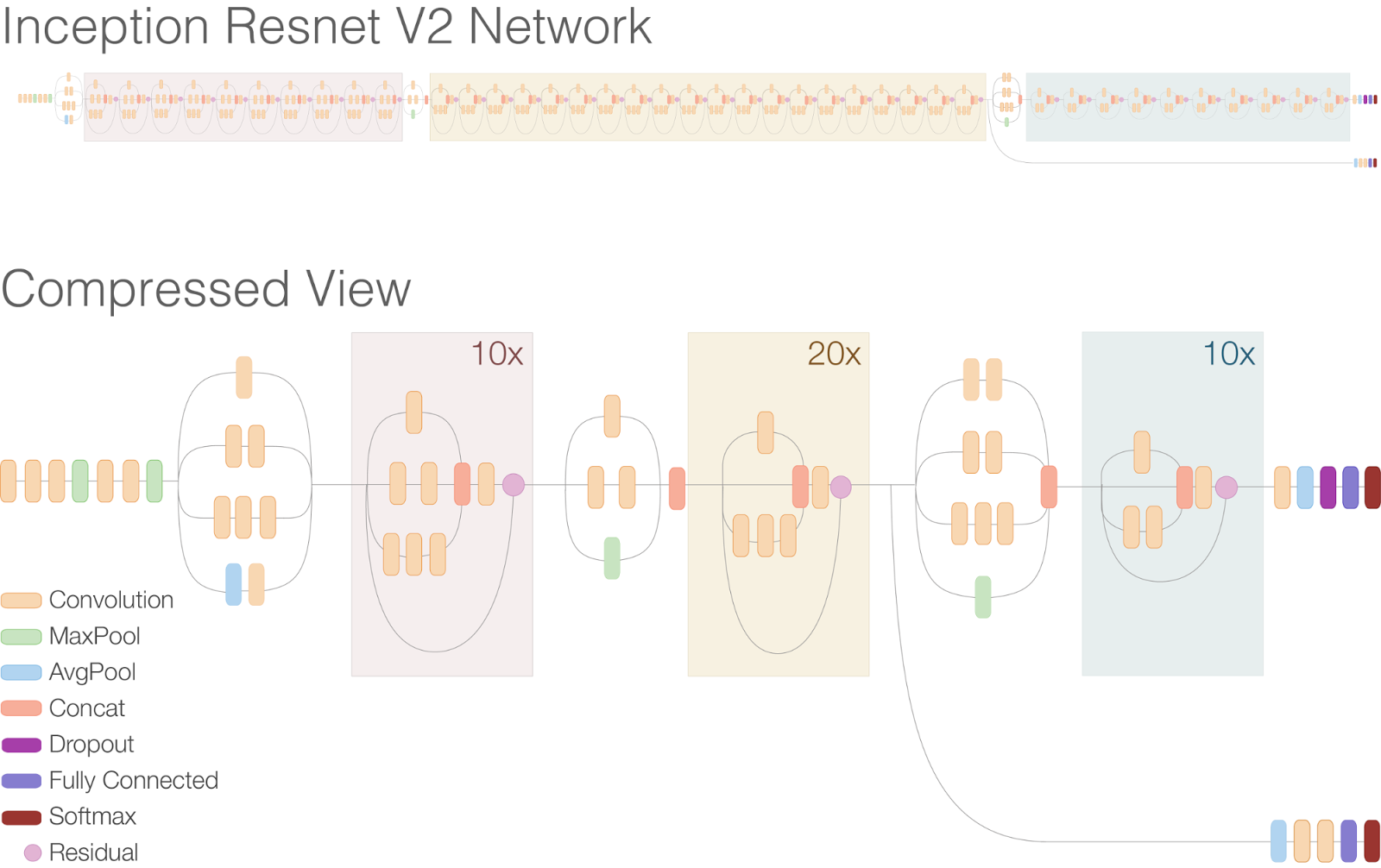Image Source: https://ai.googleblog.com/2016/08/improving-inception-and-image.html

2. Captions Data Preparation

The second part of data preparation is cleaning and transforming the captions or text Imagedata as an input to an LSTM. In the process, we conducted an exploratory data analysis of the texts as well to understand what sort of texts or images are there in the Flickr dataset.

Data Cleaning

Initially we began to work on the dataset containing 30,000 images, and once we introduced the models at a later stage of the project, we decided to use the Flickr8k subset of 8,000 images because the processing time was huge for Google Collab.

The captions prepared for LSTM input were cleaned by turning all captions to lowercase and by annotating start and end of each sequence. For VGG16 we turned the image names with .jpg into image ids.

Exploratory Data Analysis - Word Distributions

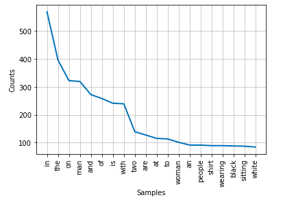
The first frequency distribution analysis of the words listed the words “in”, “the”, “on”, “man”, “and” as the most commonly occurring ones. Prepositions in any language usually belong in the realm of stop words. Stopwords can be described as the short function words, or the words that have little lexical meaning. As a preprocessing step, stop words are commonly filtered out.

NLTK.corpus contains a stopwords module that is used to easily call and eliminate function words in English language. Finally, after removing the stop words our graph of the 20 most common words in the dataset looks like this:

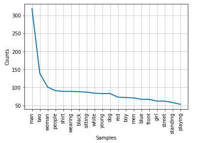
From this graph we can get an initial understanding of what the captions generally will be describing: people, young men and women, the color of their clothes, and their actions.

A weighted list of words can be represented in a word cloud, where the size of each word represents the number of its occurrences in the dataset.

Token Encoding and Sequence Modelling

All Recurrent Neural Networks (RNNs) have a chain of repeating modules of neural networks. LSTM has an advantage compared to the traditional RNN.

One of the main pain points of RNNs is short-term memory. If a sequence is long enough, they’ll have a hard time carrying information from earlier steps to the later ones. In this way RNN’s tend to leave out important information.

LSTMs are specifically designed to tackle and avoid the long-term dependency problem, thus carrying the information from previous steps is what they are designed to do. They contain “gates”, internal mechanisms that regulate the flow of information and determine which information is important to retain and leave out the non-important information.

For each image there are five captions which we turned into sequences by annotating start and end of each sequence. “startseq” starts the caption generation process. It acts as our first word when feature extracted image vector is fed to decoder. ”enseq” tells the decoder when to stop. The model will stop predicting the next word as soon as endseq appears or we have predicted all words from the train dictionary. Once this was done, we used Keras Tokenizer to transform texts to a sequence of integers.

Training the Image Captioning Decoder Model

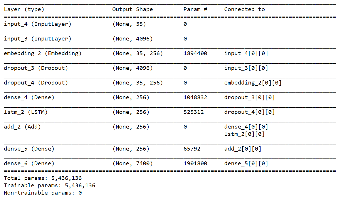
1. The Decoder Model

The image features are passed through a fully-connected layer having 256 hidden units and the captions are passed through an LSTM layer of 256 hidden units. These output vectors of two layers of size 256 are merged and passed through two dense or fully-connected layers. The final dense layer makes a softmax prediction over the entire output vocabulary for the next word in the sequence.

2. Progressive Loading using Generator Functions

Deep learning model training is a time consuming and infrastructurally expensive job which we experienced first with 30k images in the Flickr Dataset and so we reduced that to 8k images only. We used Google Collab to speed up performances using 12GB RAM allocation with 30 GB disk space available. Still, preparing the input & output sequences and corresponding the image features for the decoder model. Therefore, we started using generator functions and leveraged Keras.fit_generator

Keras.fit_generator() is used when either we have a huge dataset to fit into our memory or when data augmentation needs to be applied which precisely describes our case. With the progressive loading mechanism, the input creation part was a model training. Though model training without progressive loading couldn’t be tested for time consumption, the model training time with progressive loading took approximately 1.5 hours for five epochs and approx. 3.5 hours for 10 epochs using 6k training instances.

3. AWS Sagemaker to Scale Training Instances

Since Google Collab failed to run for a long time due to session expirations, we resorted to AWS Sagemaker for running our notebook. We used ml.t3.xlarge notebook (4 vCPU & 16 GB Memory) with 50 GB EBS Volume Size. With 5 GB EBS, the notebook was running into memory issues before progressive loading. To find more about using the right notebook instances and associated pricing, refer https://aws.amazon.com/sagemaker/pricing/.

Results

The last step of the project was to evaluate and compare the performance of the models on a hold out test set of 1000 images, using BLEU scores as a performance metric.

BLEU scores can be used to compare the closeness of a sentence to another reference sentence. The closeness is measured in terms of the number of matching tokens in both sentences and is computed by matching n-grams (i.e. matching individual words as well as pairs and sets of words), disregarding word order. A set of 4 cumulative BLEU scores is calculated for each model:

BLEU-1 - assigns the full score to matching 1-grams

BLEU-2 - assigns 50% to 1-gram and 2-gram matches respectively

BLEU-3 - assigns 33% to 1-gram, 2-gram and 3-gram matches respectively

BLEU-4 - assigns 25% to 1-gram, 2-gram, 3-gram and 4-gram matches.

As we saved a version of each model after each training epoch, we were able to evaluate the optimum number of epochs for each model as well.

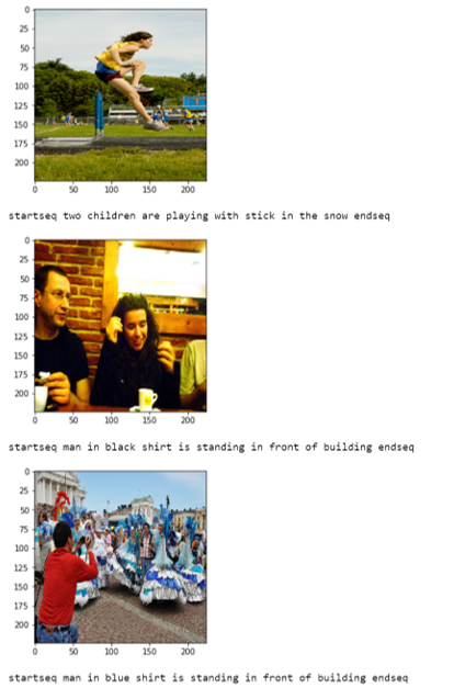
1. Evaluation of VGG16 Extracted Features

The best epoch for the model trained on VGG16 extracted image features was epoch 3 (out of 5 epochs) with the following score:

BLEU-1: 0.492964

BLEU-2: 0.238065

BLEU-3: 0.139947

BLEU-4: 0.049863

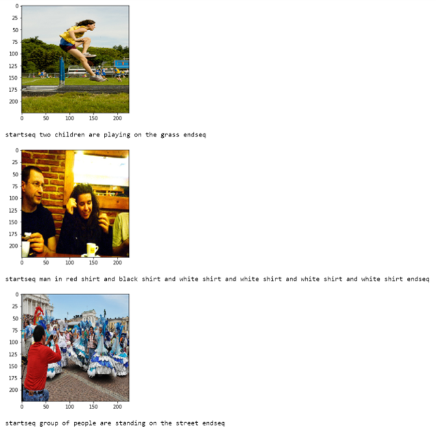
2. Evaluation of VGG19 Extracted Features

The best epoch for the model trained on VGG19 extracted features was the first epoch (out of 5) with the following score:

BLEU-1: 0.493677

BLEU-2: 0.234108

BLEU-3: 0.131691

BLEU-4: 0.043234

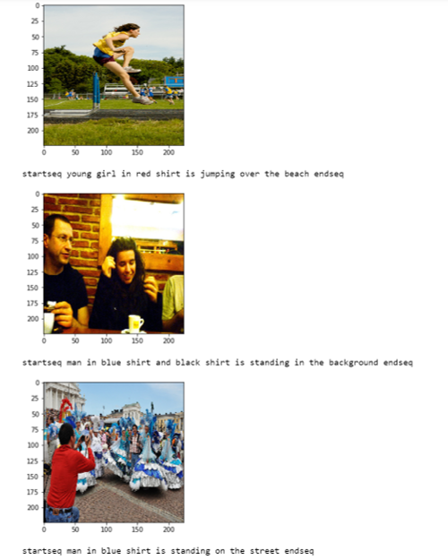
3. Evaluation of Inception Resnet V2 Extracted Features

The best epoch for the model trained on ResNet extracted features was the first epoch (out of 10), with the following score:

BLEU-1: 0.480941

BLEU-2: 0.221203

BLEU-3: 0.126065

BLEU-4: 0.041060

Conclusion

The project was really helpful in understanding how CNNs work to identify image contents. We used pre-trained models like VGG and Inception_Resnet_v2 to extract image features and so we learnt about their architectures and how they work. To train and predict image captions, we also worked on implementing LSTM and some basic cleaning texts using Natural Lanaguage Processing techniques. One the basic challenges all the way was to process so many images and extracted features which forced us to move towards cloud infrastructure. Most of us also were coding for the first time with Keras and thus this was a great hands-on practice on coding deep learning models using Python & Keras modules, especially how to work with generator functions and how they are used to overcome big data challenges.

WaiPRACTICE

Contributors